Today for my IBM project I wanted to learn more about imputation methods, selection of features, types. The following is from Flexible Imputation of Missing Data by Stef Van Buuren .

Types of Missing data

Let $D = {(x,y)^i}$ and $X$ be our missing data column where $X := (X_{obs}, X_{missing})$ for $\theta$ being the parameter of missing values then;

(1)Missing completely at random (MCAR) - Unlucky out of control missing values that is \(Pr(R = 0 |X_{obs}, X_{missing}, \theta) = Pr(R=0| \theta)\) .

(2)Missing at random (MAR) - through our asusmption of sampling, data is missing that is \(Pr(R = 0 |X_{obs}, X_{missing}, \theta) = Pr(R=0| X_{obs}, \theta)\) .

(3)Not missing at random (NMAR): \(Pr(R = 0 |X_{obs}, X_{missing}, \theta)\).

Commonly used Imputation are Problematic

Method 1 : (Complete Case Anlysis) - deleting samples why any features missing

Revmoing all samples where there is a missing input. that is if i have D = (200, 30) if one of the index = 189 has one missing values in column = 5 then i would remove the whole index, but even thoruhg removing missing values is fast this assume missing data is MCAR,. If this assumption is not true then by removing these missing values is casue estimators for future paramettric models, such as linear regression etc to have bias estimators of (1) mean, (2) regression coefficients (3) correlation.

Method 2: Avaliable Case Anlalysis - not deleting any missing entries

If we are anylysing two features $X_1$ and $X_2$ if both features have different index where data is missing, we don’t remove them missing values. Problems with this method is it assume missing values are MCAR, thus if the assumption is wrong then it bias estimators of future learning models. Secondly, sample size could be different for each category being analysed, leading to complication of analysis of whole dataset.

Method 3: Mean Imputation

For each features the mean is taken then is placed into each missing values of that coloumn. The problem with this reguards of the type of missing data, this distors the variance. Also if tehre is a positive correlation between vairables then it icnrease the correlation by using eman imputation

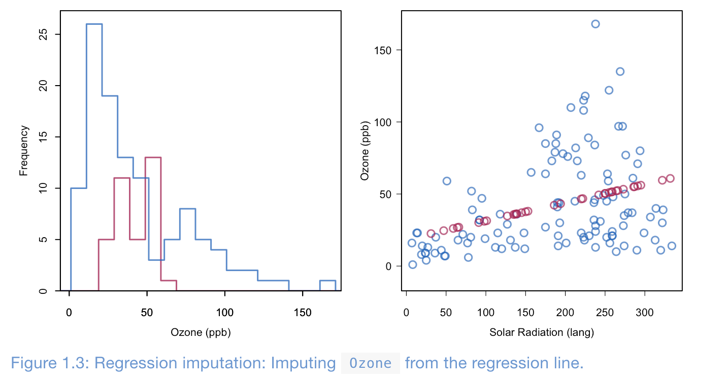
Method 4: Regression Imputation

Viaselection some slection method, we can compute univairate or multivairate regression and then use this information to fill in the missing values. Importantly we are not interpolation each data points, but rather estimated via dataset. The benefits of this method is if the data is MCAR or MAR has unbias estimatros for future parametirc learning models, but by using the relationship between variables and inputing these values into missing data point, we icnrease the correlation between the used features vairables in the regression model. Addtionally, it decrease the samples variables in sample, thus cause underestimation of variatability.

Even though this is the most commonly used method for imputation is it extremelt dagerous due to increased correlaotion (relation) between vairables, which cause more false positives in future learning models.

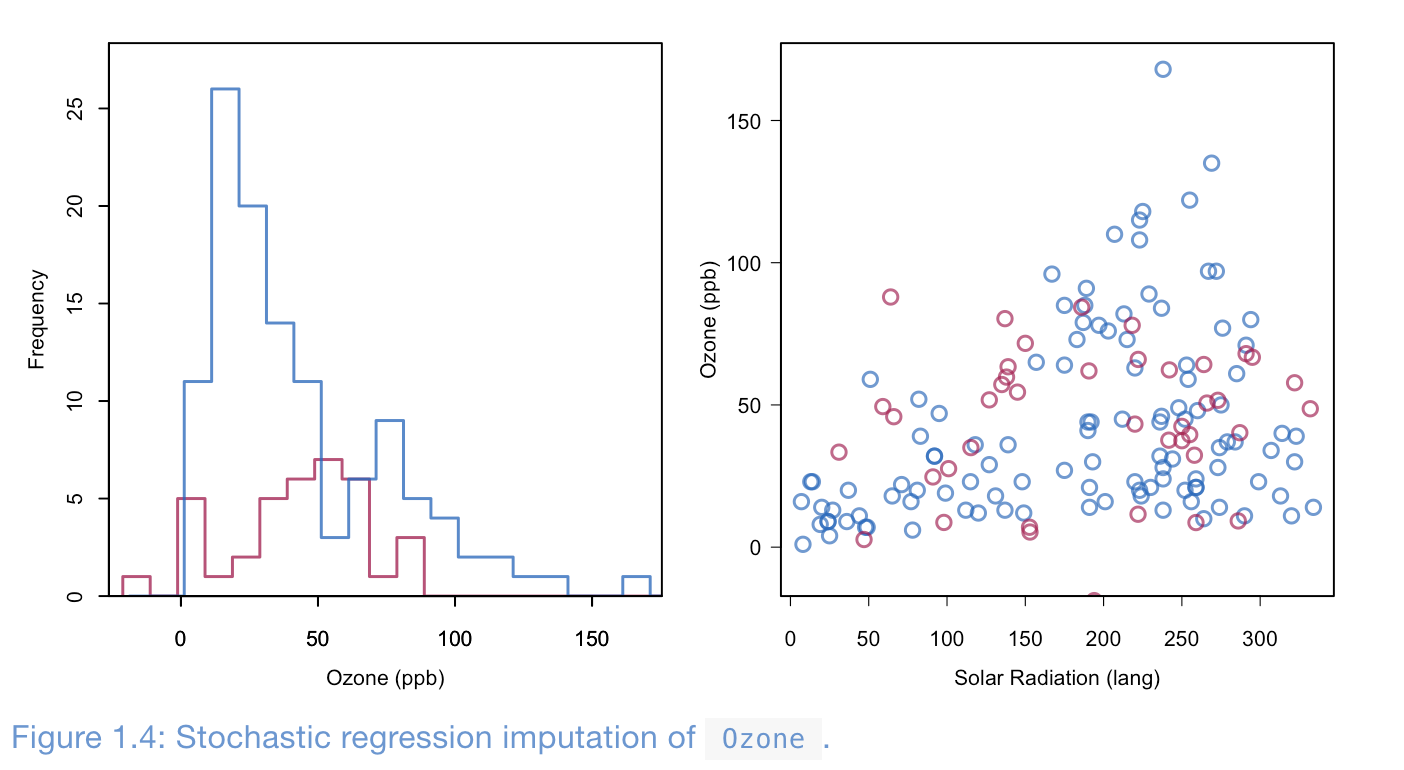
Method 5: Stochastic regression imputation (SRI)

Doing Regression Imputation, but now we add noise to decrease correlation bias.

Even thought the benfits of this model is it does not underestimate the variance, it has larger sample variacne of estimators then compared to other imptuation. Addtionaly, the standard error of learning models using on features using SRI n have are very small, thus dont adress uncertainty of estimation! Continuing, SRI genrally doesnt adress higher end of frequency, can randomly assign noise negative values even thought it might not be plausible (weight can be negative)

Summary of Commonly used Imputation methods

All these methods have inherent problems, effecting bias of future learning model estimators or not identifying the correct distribution. All the methods above are known as single imputation, that it they only given a method mean imputation, SRI imputation they all predict a single data value for each missing data point. Whihc increases biais since how do we know that our current sample is a accurate representation of the whole population/distribution?

Current Solutions to imputations : Multiple Imputation

Multiple Imputation

Generally when we conduct supervised learning we can do it with one feature (X, Y) or with multiples features to predict one label.

Univariate Multiple Imputation

this is the case when we only have missing values in one feature, there are two types

Univariate Multiple Imputation : Continuous Feature

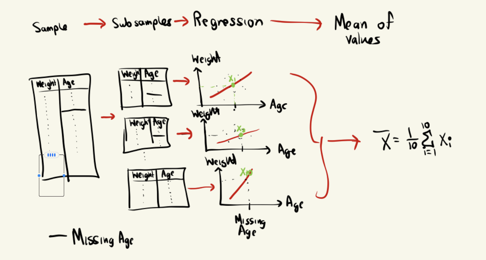
An example, suppoer we have a dataset, where the columns are weight, eye_colour, nationality, age, income, Body Mass Index, height. Suppose we want to want to make a classification algorithm to find the height of someone. So the potential features are weight, eye_colour, nationality, age, income, BMI. From a basic data profiling we find that age has a missing value in index 10. So what we can do is we find the correlation between (weight and age) have a high correlation, thus we use so what we do first is we split our dataset into say 10 parts. Then we conduct any learning model like regression, linear or non linear. Then from our subsamples we predic the missing values of age. Thus we have 10 different values for age in index 10, then we can one method is to compute the mean of all these estimates for age at index 10 and thus we have now reduced our bias, but using in a sense multiple samples from the unknown distribution, rather then computing it from one sample. The figure brlow illustrates this idea,

There are 4 main types of models to estimate the missing index via subsamples (not the missing column) is normally distributed

1. Regression Imputation - $$ \hat{y} = \hat{\beta_{0}} + X_{missing}\hat{\beta_{1}}
2. Stochastic Imputation \(\hat{y} = \hat{\beta_{0}} + X_{missing}\hat{\beta_{1}} + \epsilon\) where \(\epsilon ~ N(0, \sigma^2)\)
3. Bayesian multiple imputation - \(\hat{y} = \hat{\beta_{0}} + X_{missing}\hat{\beta_{1}} + \epsilon\), but now rather the above assume frequentist statistics, we use Bayesian Statistics and assume our parameters, \(\hat{\beta_{0}}, \hat{\beta_{1}} \text{ and } \sigma\) are from some posterior distribution we have chosen.
4. Bootstrap Multiple Imputation

Note when our \(\hat{y}\) is not normally distributed then we conduct a transformation to make it normally distributed.

Univariate Multiple Imputation : Categorical Feature

In this case we use generalized linear models, specifically logistic regression, for binary classes

Multi-class using, multinomial logit model for nominal categorical variables

Ordered Logit Model for ordinal categorical variables

\(\begin{align*} Pr(y_i \leq K | X_i, \beta, \tau_k) = \frac{\exp( \tau_k - X_iB)}{1 + \exp( \tau_k - X_i\beta)} \end{align*}\) so for a given category

Multiple Multiple Imputation

THre problem wit the above example is that in the real world missing data span different index’es and multiple features, so

• Imputation stronger if not multiples variables are missing for each data
• Measuring Usability of dataset when multiple missing coloumns and index
  • Proportion of usable cases
  • Outbound Statistic, Inbound statistics (for two features measure )
  • Influx and outflux coefficient (comparison of Outbound Statistic, Inbound statistics for multiple featrues )
• Issues
  • predictors contain missing values
  • Variables are often of different types
  • collinearity can occur
  • he ordering of the rows and columns can be meaningful, e.g., as in longitudinal data
  • the relationshiup between variables can be non-linear
  • Imputation can create impossible combinations, such as pregnant fathers.
• Methods
  • Monotone data imputation. (MICE) For monotone missing data patterns, imputations are created by a sequence of univariate methods;
  • Joint modeling. For general patterns, imputations are drawn from a multivariate model fitted to the data;
  • Fully conditional specification, also known as chained equations and sequential regressions. For general patterns, a multivariate model is implicitly specified by a set of conditional univariate models. Imputations are created by drawing from iterated conditional models.
• Analysing Imputation
  • Workflows
  • dont use for pool part :
    • Average Mean -> incorrect standard errors, confidence intervals and p-values -> wrong statistical testing or uncertainty analysis
    • Stack imputed data ->
  • Use:
    • Repeated analyses
  • Identify the best features for imputation: problem when using stepwise model selection:
    • When seperated data in subsamples then, The first step involves performing stepwise model selection separately on each imputed dataset, followed by the construction of a new supermodel that contains all variables that were present in at least half of the initial models.
    • Majority. A method that selects variables in the final that appear in at least half of the models.
    • tack. Stack the imputed datasets into a single dataset, assign a fixed weight to each record and apply the usual variable selection methods.
    • Wald. Stepwise model selection is based on the Wald statistic calculated from the multiply imputed data.

Application

• Chosing which imputation model (regresion type etc after subsamples) is hardest choice ou goals is to
  • account for the process that created the missing data,
  • preserve the relations in the data, and
  • preserve the uncertainty about these relations.
• Choise we need to make
  • MAR assumption is plausible ?
  • form of the imputation model. The form encompasses both the structural part and the assumed error distribution?
  • set of variables to include as predictors in the imputation model. The general advice is to include as many relevant variables as possible, including their interactions
  • impute variables that are functions of other (incomplete) variables (like my time diff/ratio’s)
  • the order in which variables should be imputed.
  • setup of the starting imputations and the number of iterations
  • The number of multiply imputed datasets
• Generally
• The MAR assumption is often a suitable starting point. If the MAR assumption is suspect for the data at hand, a next step is to find additional data that are strongly predictive of the missingness, and include these into the imputation model. If all possibilities for such data are exhausted and if the assumption is still suspect, perform a concise simulation study as in Collins, Schafer, and Kam (2001) customized for the problem at hand with the goal of finding out how extreme the MNAR mechanism needs to be to influence the parameters of scientific interest. Finally, use a nonignorable imputation model (cf. Section 3.8) to correct the direction of imputations created under MAR. Vary the most critical parameters, and study their influence on the final inferences. Section 9.2 contains an example of how this can be done in practice.
• In my experience, the increase in explained variance in linear regression is typically negligible after the best, say, 15 variables have been included. For imputation purposes, it is expedient to select a suitable subset of data that contains no more than 15 to 25 variables. provide the following strategy for selecting predictor variables from a large database:
  • Include all variables that appear in the complete-data model, i.e., the model that will be applied to the data after imputation, including the outcome (Little 1992; Moons et al. 2006). Failure to do so may bias the complete-data model, especially if the complete-data model contains strong predictive relations. Note that this step is somewhat counter-intuitive, as it may seem that imputation would artificially strengthen the relations of the complete-data model, which would be clearly undesirable. If done properly however, this is not the case. On the contrary, not including the complete-data model variables will tend to bias the results toward zero. Note that interactions of scientific interest also need to be included in the imputation model.
  • In addition, include the variables that are related to the nonresponse. Factors that are known to have influenced the occurrence of missing data (stratification, reasons for nonresponse) are to be included on substantive grounds. Other variables of interest are those for which the distributions differ between the response and nonresponse groups. These can be found by inspecting their correlations with the response indicator of the variable to be imputed. If the magnitude of this correlation exceeds a certain level, then the variable should be included.
  • In addition, include variables that explain a considerable amount of variance. Such predictors help reduce the uncertainty of the imputations. They are basically identified by their correlation with the target variable.
  • Remove from the variables selected in steps 2 and 3 those variables that have too many missing values within the subgroup of incomplete cases. A simple indicator is the percentage of observed cases within this subgroup, the percentage of usable cases (cf. Section 4.1)
  • In practice, there is often a small set of key variables, for which imputations are needed, which suggests that steps 1 through 4 are to be performed for key variables only. The mice package contains several tools that aid in automatic predictor selection. The quickpred() function is a quick way to define the predictor matrix using the strategy outlined above. The flux() function was introduced in Section 4.1.3. The mice() function detects multicollinearity, and solves the problem by removing one or more predictors for the model.
• Say our time_diff = based on end_time and start_time if we impute all these values we will have values for that index which don’t make sense, The easiest way to deal with the problem is to leave any derived data outside the imputation process.
• Conditional imputation : In some cases it makes sense to restrict the imputations, possibly conditional on other data. The method in Section 1.3.5 produced negative values for the positive-valued variable Ozone. One way of dealing with this mismatch between the imputed and observed values is to censor the values at some specified minimum or maximum value. The mice() function has an argument called post that takes a vector of strings of R commands. These commands are parsed and evaluated just after the univariate imputation function returns, and thus provide a way to post-process the imputed values. Note that post only affects the synthetic values, and leaves the observed data untouched. The squeeze() function in mice replaces values beyond the specified bounds by the minimum and maximal scale values. A hacky way to ensure positive imputations for Ozone under stochastic regression imputation is
• Interaction terms
• Quadratic relations Algorithms type
  • Visit sequence
  • Convergence Diagnostics
  • Model fit versus distributional discrepancy
  • Diagnostic graphs